Machine Learning Optimization · Research Paper

ML-Driven Rolling Horizon Optimization

Combining LSTM-based deep learning forecasting with Stackelberg game theory for data-driven building-to-building energy exchange decisions.

Journal: IEEE Transactions on Industry Applications (2025)

Authors: M.B. Gebremariam, P. García, Á. Navarro-Rodríguez, Ó. Pasarín, C. Blanco

Data: 4 buildings · Barcelona, Spain · 15-min & 1-hour resolution

Rolling Horizon LSTM-Based B2B Optimization

This research combines the predictive capability of LSTM-based machine learning with Stackelberg game theory to create a rolling-horizon energy exchange optimisation system. Buildings make informed, profitable trading decisions by forecasting PV generation and load demand 24 hours ahead — adapting in real time to dynamic building energy patterns.

LSTM Deep Learning Rolling Horizon Stackelberg Game 24h Forecasting ESS Degradation Scalability

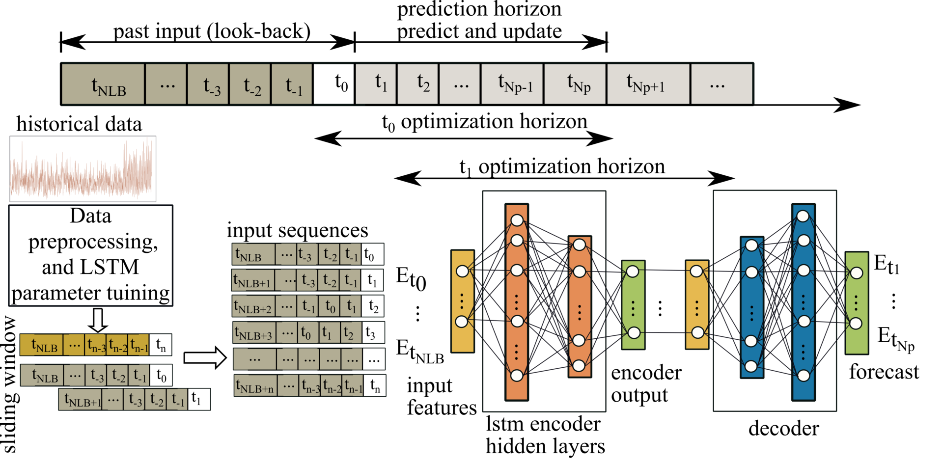
LSTM Architecture — **Fig. 3.** General structure of the LSTM model for rolling-horizon energy exchange, showing the encoder-decoder architecture with sliding window input and multi-step forecast output.

How the Forecasting Works

An encoder-decoder sequential LSTM model with multiple layers generates 15-minute and 1-hour resolution forecasts of PV generation and load demand for each building. The model uses a sliding window approach with customisable look-back periods — recognising that each building has unique energy patterns requiring tailored hyperparameters.

Forecasting Performance

Hyperparameter Tuning

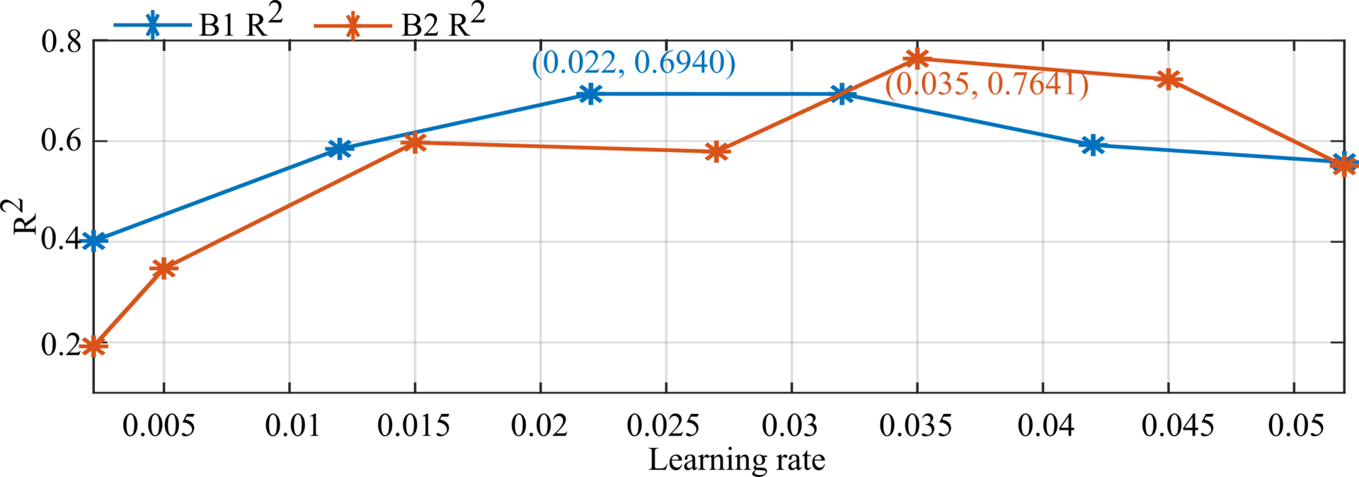
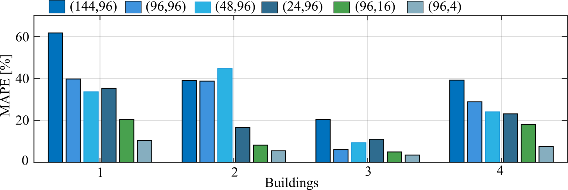
Each building receives a customised LSTM configuration: look-back window, layer count, learning rate, and forecast sequence length are individually optimised via grid search, achieving significantly lower MAPE than one-size-fits-all approaches.

Load & PV Forecasting

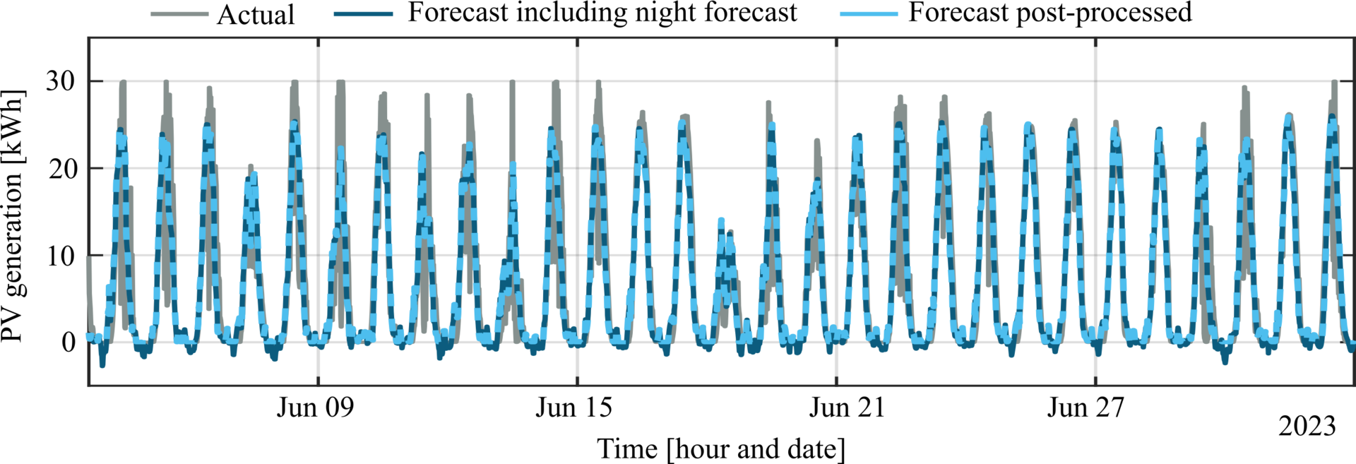
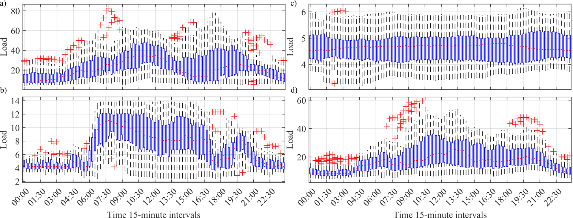
Buildings 1 and 4 exhibit higher loads and greater variability, while Building 3 has a more consistent pattern (lowest MAPE: 6.07%). PV forecasting uses post-processing to replace nighttime values with zero, achieving high accuracy for the critical 24-hour ahead window.

Load Profiles — **Fig. 6.** Box plots of 15-minute load profile test data for each building, revealing different variability and demand patterns.

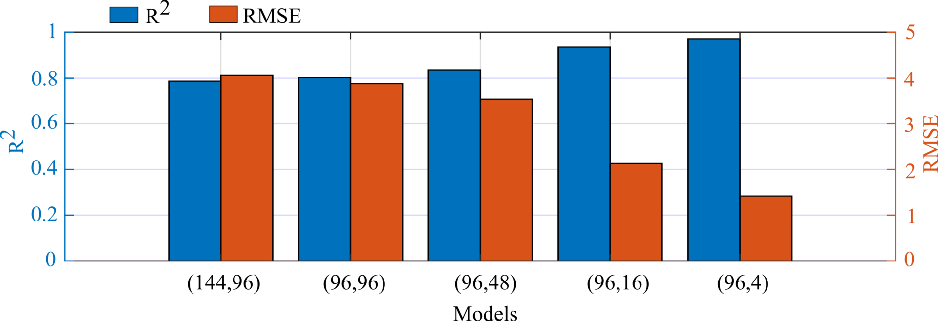
PV Accuracy — **Fig. 8.** PV forecasting accuracy with different models at 15-minute resolution; accuracy increases as the forecasting period decreases.

PV Forecasting — **Fig. 7.** PV generation forecasting comparison (96-sample look-back, 96-sample forecast) — actual vs. raw forecast vs. post-processed forecast with nighttime correction.

Rolling Horizon Energy Exchange Results

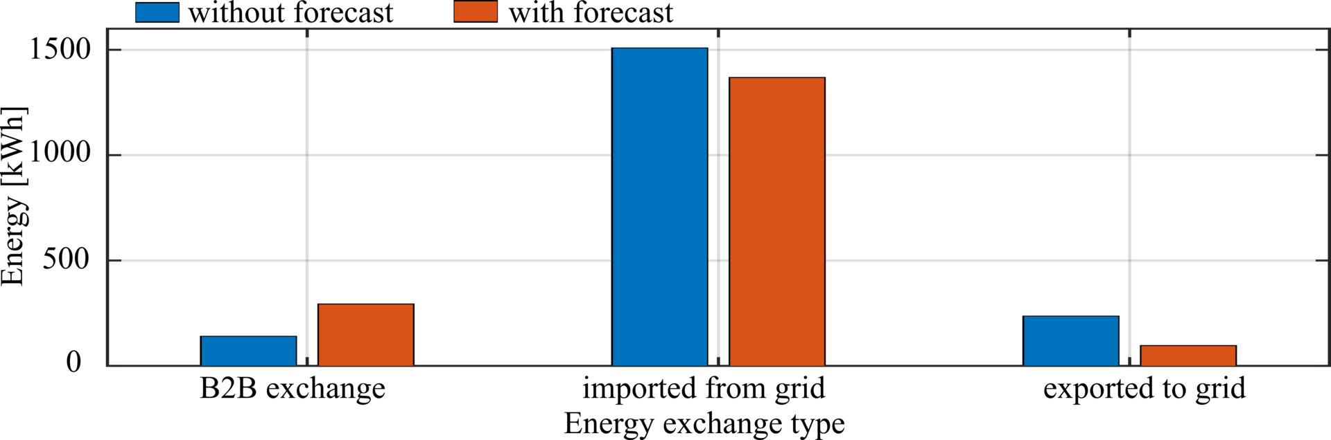
The proposed model is compared against three scenarios: game theory without forecasting, with LSTM forecasting, and with perfect (100%) forecasting. As prediction accuracy improves, energy costs decrease — validating the critical role of ML in B2B trading.

Key Performance Metrics

2.67–29%

Cost saving with LSTM forecast

3.33–59%

Cost saving with perfect forecast

€4,993

Max yearly saving per building

4 → 32

Buildings with fast convergence

Exchange Comparison — **Fig. 12.** Energy exchange comparison with and without forecasting — increased B2B exchange and reduced grid imports with the LSTM model.

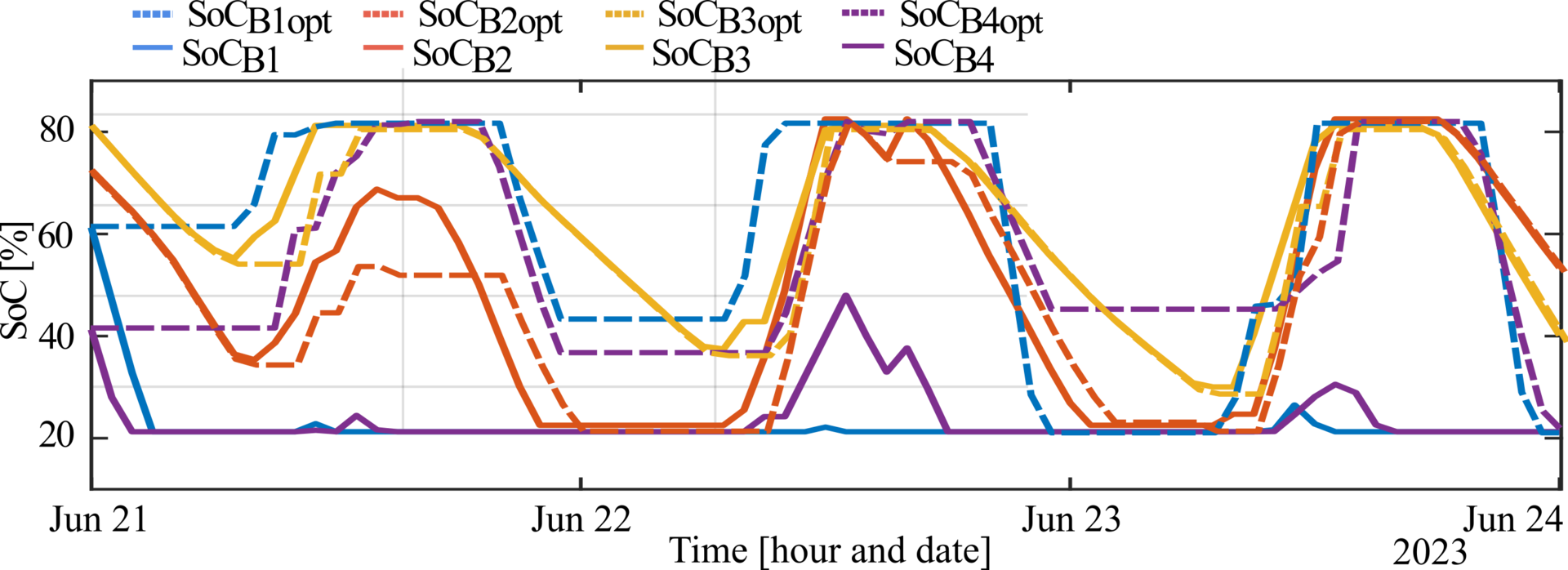
**Fig. 14.** ESS SoC results with (dashed) and without (solid) forecasting — forecasting increases ESS participation in the B2B network.

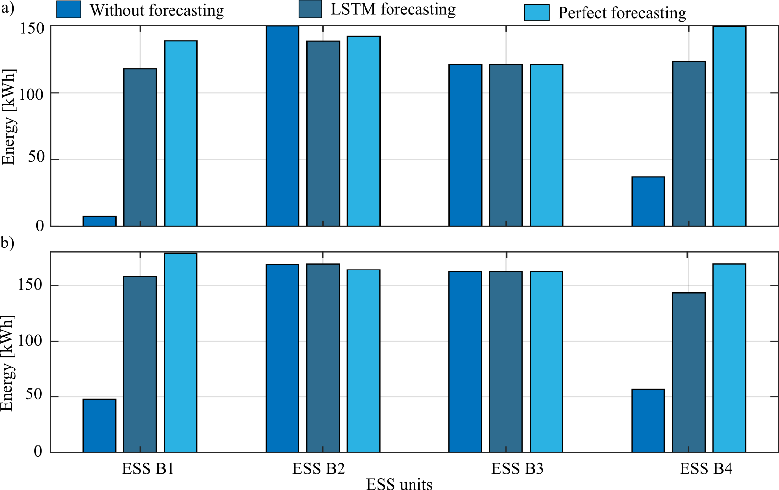
ESS Comparison — **Fig. 15.** Total energy charged and discharged at each building ESS: comparing no-forecast, LSTM forecast, and perfect forecast scenarios.

Sensitivity & Scalability

ESS Capacity Impact

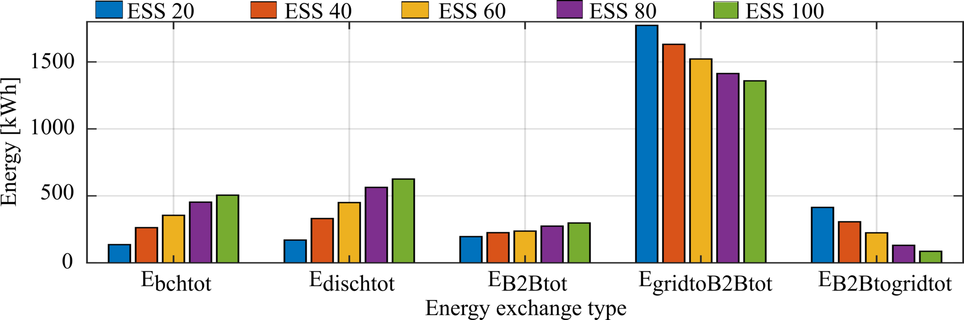
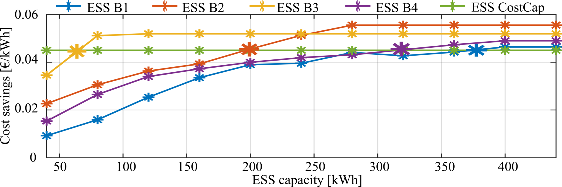
The sensitivity analysis examines ESS capacities from 20 to 100 kWh. Higher capacities increase B2B autonomy and reduce grid dependence, but moderate capacities (60–80 kWh) offer the best balance between cost savings and investment return.

Energy vs ESS — **Fig. 16.** Total energy exchanged as ESS capacity changes from 20 to 100 kWh, showing increased autonomy with larger storage.

Cost vs ESS — **Fig. 17.** Cost savings vs. ESS capacity — asterisks mark where storage becomes profitable for each building.

Network Scalability

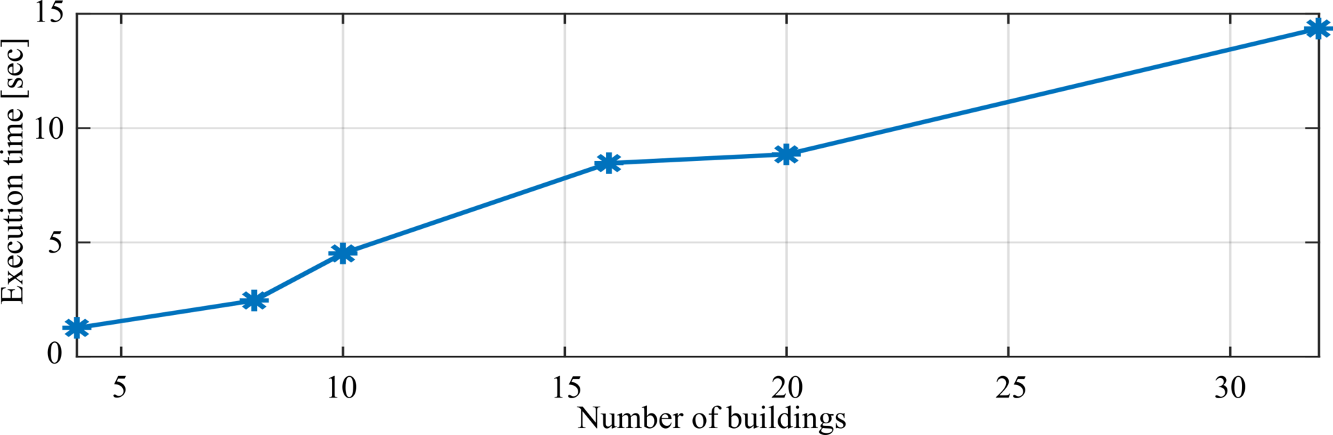
Tested from 4 to 32 buildings, execution time scales from 1.26 to 14.35 seconds — demonstrating practical feasibility for real-time B2B market operation. B2B energy exchange and ESS utilisation increase proportionally while maintaining consistent per-building savings.

Full paper citation:
M.B. Gebremariam, P. García, Á. Navarro-Rodríguez, Ó. Pasarín, C. Blanco, "Building-to-Building Grid Energy Exchange Optimization: A Rolling Horizon Game Theory Approach with Machine Learning Forecasting," IEEE Transactions on Industry Applications, 2025.

DOI: 10.1109/TIA.2025.3645147 ↗